The purpose of this article is to introduce the reader into time series analysis field. We will focus on emphasizing the difference between time series and other forms of data and we will introduce selected data science methods useful in time series analysis.

What is a time series? 

Time series is any set of data points, that could be indexed in time order. For example it could be a series of speed measures of passing cars, with two values for each “data point” - speed and timestamp. The format in which the time is recorded is irrelevant. It could be number of seconds since 01.01.1970 or any other representation. But how is time series different from other datasets?

Let us get back to the example with speed measures. One of the first steps of analysis could be calculating mean and standard deviation of speed, and if we take the timestamp, we can calculate this value for every hour separately, which can determine, at which time of the day drivers are more likely to exceed the speed limit, or on which days the traffic is higher than usual.

Time domain gives the data analyst whole range of possibilities to draw interesting conclusions.

Dataset

In this  article we will use a dataset coming from kaggle, titled “Advance Retail Sales Time Series Collection”. It consists of 28 different series, describing sales of certain product groups, such as apparel, food or garden tools. In this example the measurements are evenly spaced, but it’s not a requirement. To start with, we will plot the series. What is interesting is the tremendous variety of their shapes.

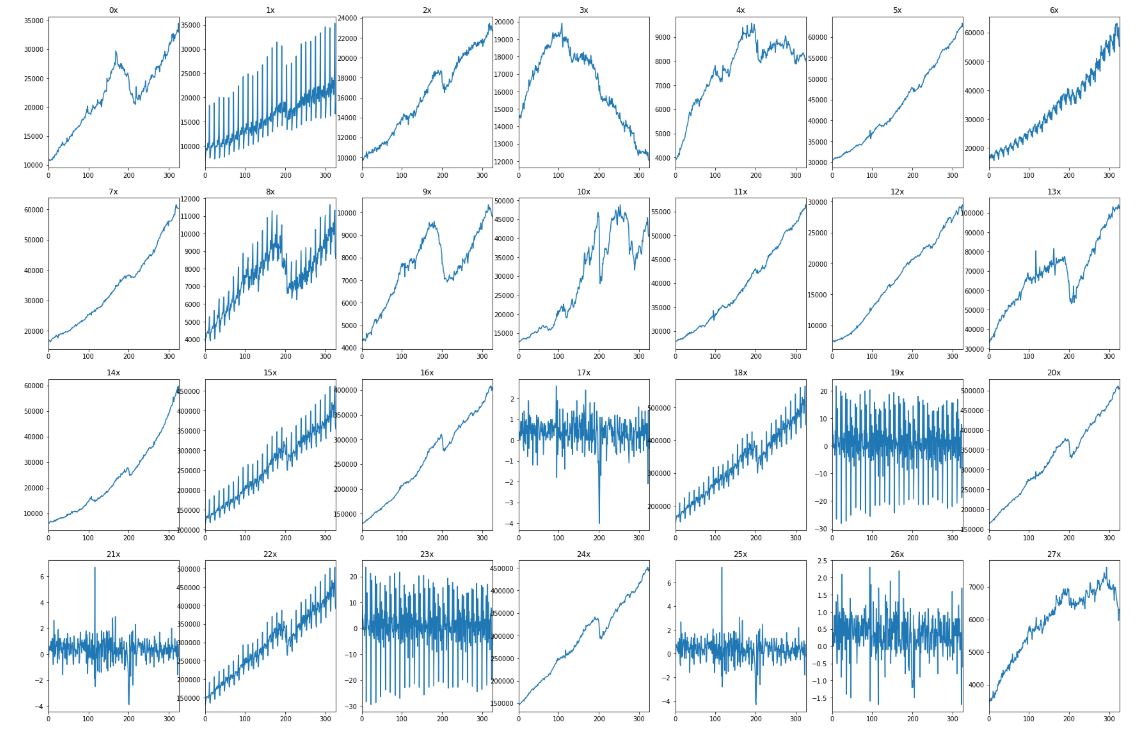
Some of them are strictly increasing, some do change the direction, the rest is oscillating around some specific value. We will zoom in to chart “6x”, located in upper right corner:

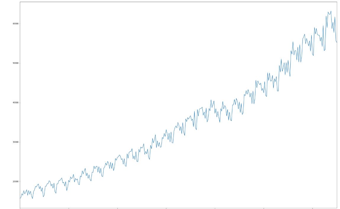
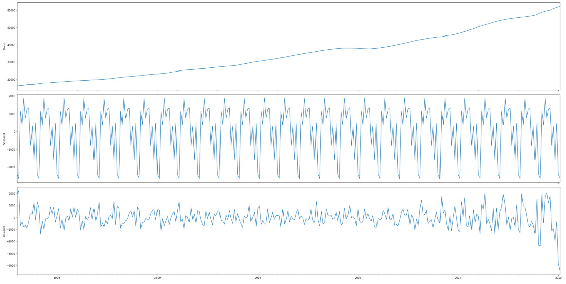
What can we say about it? First, value of the series grows over time. Apart from the upward trend, which we can aproximate with a linear of polynomial function, a second component is a series with strong seasonality. Standard method to analyse time series is to decompose it into a combination of three components: trend (in this case nonlinear), a periodical part (seasonality) and residue – noise.

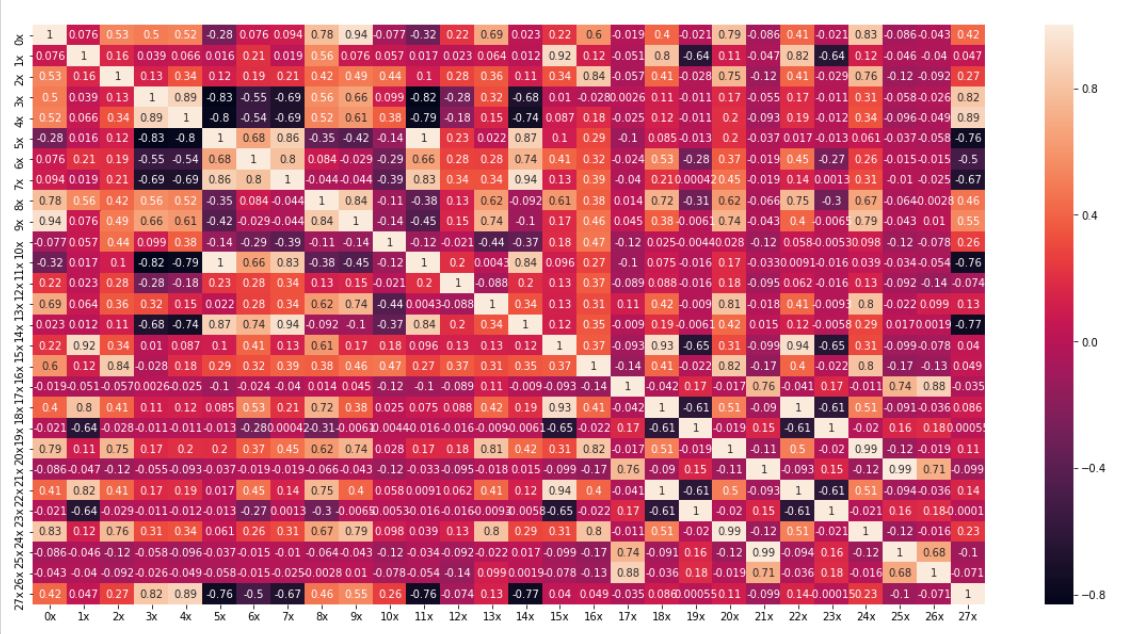
Value of trend is a one order of magnitude higher than other components and it has a big influence on correlation between series, because most of them contain similar trend. On the first chart we can see the correlation values for unchanged series:

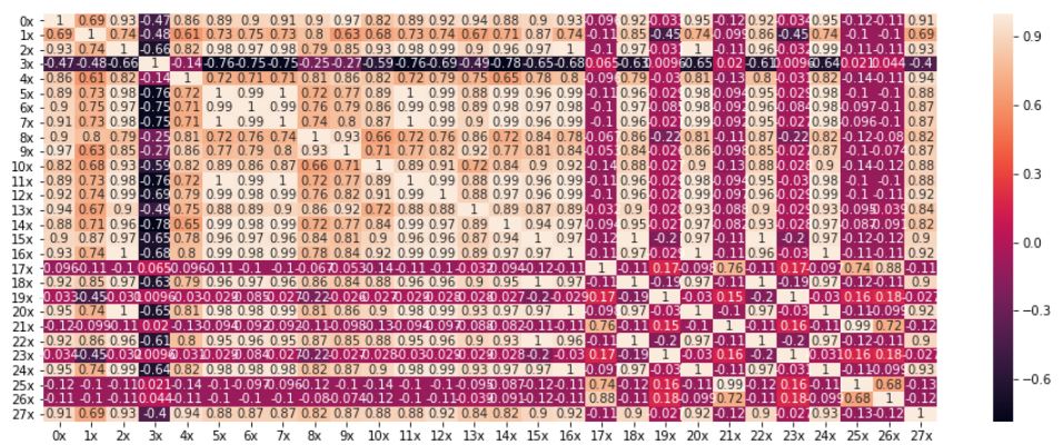
In this case first 17 series are strongly correlated, some values are equal to 1, which means that the files contain exactly the same data, just possibly linearly scaled. Correlation matrix of detrended series (with linear approximation of trend function) looks quite different:

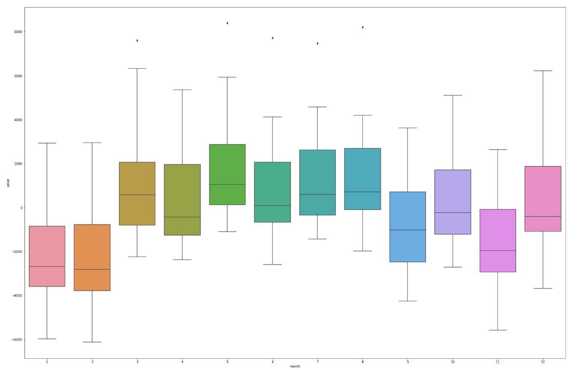
Behind most of the relationships was continously rising sales (trend), correlations caused by seasonal component and residue are much less frequent. Trend removal enhances the local features of the series. Let us take axample of sales grouped by month:

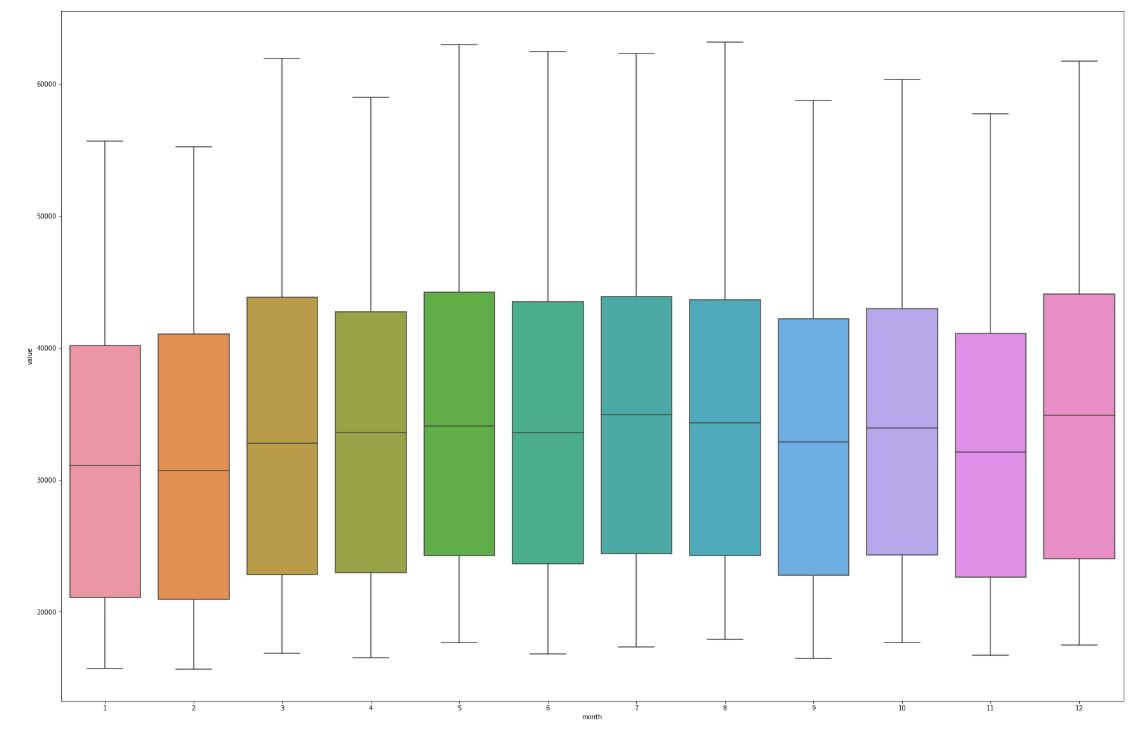
Much more interesting is the same chart, but plotted for detrended series. The differences between months are much more significant.

Seasonality analysis

For the purpose of seasonality analysis we have few more methods to use, for example autocorrelation function. It is calculated as follows: n-th term is a correlation coefficient of original series with series shifted by n steps. The idea can be illustraded with sine function. Shifting it by n elements is just applying the phase shift of n. Calculating the correlation will show us how much the shifted sine is similar to original series. If the shift will be equal to it’s interval, correlation will  be equal to 1.

Confidence intreval for autocorrelation function

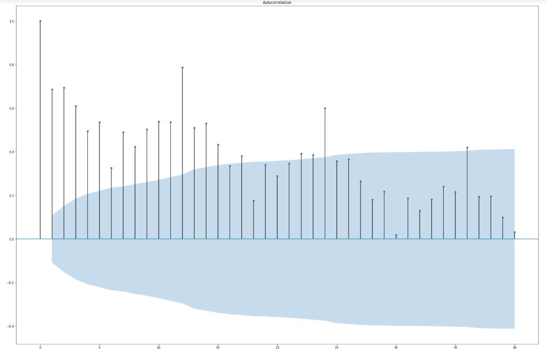
How to determine, whether correlation is caused by series property, not just plain coincidence? Blue area on chart below is 95% confidence interval. It means, that if the correlation value exceeds it, we have >95% of confidence, that it is significant. It is of course a simplified interpretation. Below we limited the chart to shift by 40 steps. As we can see, the function has maxima every 12 steps (months),  periodicly. It is another visual evidence of periodicity of sales in an annual cycle.

Stationariness of time series

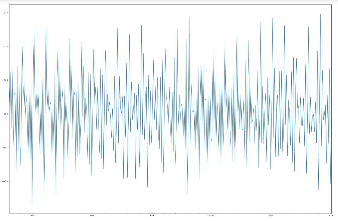
The last issue we would like to discuss is stationariness. Series (or underlying stochastic process) is stationary (or formally: wide-sense stationary) if its mean, variance and autocorrelations are not time dependant. Series “6x” is of course non stationary because of the visible trend and seasonality, which affect mean value. Stationary time series are much easier in analysis, many of popular models actually require to transform the series into a stationary form. Depending on the underlying reason of nonstationariness, we can use different methods of transformation. One of them, removing linear trend is to replace series Y[0], Y[1], … Y[n] by differences in a form X[0] = Y[1] – Y[0]. After such transformation, our series looks as below.

Stationariness verification

As we can see, we got rid of the trend. Is that enough to render the series stationary? We cannot forget about seasonal component, which might be significant enough to remove it. As in the autocorrelation function, there are statistical methods allowing to assess the significance of seasonality. For example, theres a KPSS statistical test, named after names of its authors: Kwiatkowski–Phillips–Schmidt–Shin.

Typical form of a statistical test goes as follows. We form two hypotheses – hull hypothesis - which states, that our series is stationary and alternative hypothesis, which claims the contrary. We choose a confidence interval, usually it is 95%. We have to remember that we are considering random numbers, not a function given with its formula, so we always talk about probability, not certainty. 

The statistical test itself is comparison between so called test statistic and its critical value, determined by confidence interval we want to obtain. The test statistic is computed (by your favourite software), but it is important to understand its interpretation and implications. If the test statistic value is higher than the critical value, we have to reject the null hypothesis, therefore our series is not stationary.

Summary

After reading this post, the concept of time series should be more familiar. We have learned to transform it and decompose it into components as trend and seasonality. At the end we have intoduced the concept of stationariness. We know how to transform some series into a stationary form and how to check the statistical significance. We should be ready now to model the series for predictive purposes!